Bulk 구조 및 Ring 구조에서의 결합계수를 구하는 것은 이전 글을 참고하기 바란다.
To find the coupling coefficients for Bulk and Ring structures, see the previous article.
CST STUDIO SUITE Learning Edition - Low Frequency Solver를 이용한 결합계수(Coupling Coefficient) 계산하기(Calculatio
기본적인 Coil의 인덕턴스(Self inductance)를 해석하는 것은 이전 글을 참조하기 바란다. https://mwave.tistory.com/312 CST STUDIO SUITE Learning Edition - Low Frequency Solver를 이용한 WPC Qi A11 Coil(Wireless Charging) 해석하
mwave.tistory.com
Self Inductance 계산 예는 다음과 같다.
An example of a self Inductance calculation is shown below.
CST STUDIO SUITE Learning Edition - Low Frequency Solver를 이용한 WPC Qi A11 Coil(Wireless Charging) 해석하기
WPC Qi A11 Coil 의 세부 구조는 하기의 링크를 참조하기 바란다. https://mwave.tistory.com/310 WPC Qi 규격 중 BPP A11 코일 및 시스템 사양에 대하여 일반적으로 WPC Qi의 A11 교격은 5W 무선충전기에서 가장 많이
mwave.tistory.com
Learning Edition에서 Spiral 구조에서의 결합계수가 기존 방식에서 mesh 수의 제약으로 해석이 안되었다. 계산 정밀도를 낮추니 해석이 가능해서 결과를 공유한다. 다만 결과치가 정상적인 부분보다 값들이 낮게 나오니 감안해야 하고 경향성만 본다고 생각해야 한다. 여기서 코일간 거리는 3mm를 기준으로 하였다.
In the Learning Edition, the coupling coefficient in the spiral structure could not be analyzed due to the limitations of the mesh number in the existing method. By reducing the calculation precision, it can be interpreted, so we share the results. However, the results are lower than the normal part, so you should consider it and think of it as a trend. Here, the distance between the coils was based on 3mm.


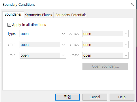
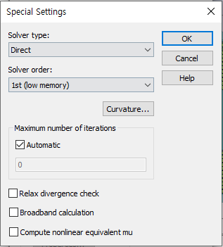
Solver에서 Special Setting 기준 Solver order를 1st(low memory)로 설정하면 mesh수를 63,333미만에서 해석 가능합니다.
If you set Solver order to 1st (low memory) under Special Setting in Solver, the mesh count can be solved at less than 63,333.

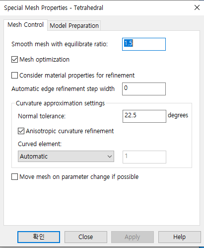
이 결과 mesh 수는 33,393개이고, 20,000개를 초과했음에도 해석 결과를 얻을 수 있다. 다만 정확도는 떨어진다. 정상적인 해석보다 수 uH 낮게 결과가 나온다.
This results in a mesh count of 33,393, and we can still get results despite exceeding 20,000 meshes. However, it is less accurate. The result is several uH lower than a normal analysis.


Self inductance 값이나 Coupling Coefficien 값이 조금 낮게 나왔으나 경향성만 참고한다면 이 방법도 이용할 가치는 있다고 생각된다.
The self inductance and Coupling Coefficien values are a bit lower, but I think it's worth using this method just for the trend.
이상 글을 마친다.
That's all for now.


댓글