WPC Qi A11 Coil 의 세부 구조는 하기의 링크를 참조하기 바란다.
For the detailed structure of WPC Qi A11 Coil, please refer to the link below.
WPC Qi 규격 중 BPP A11 코일 및 시스템 사양에 대하여
일반적으로 WPC Qi의 A11 교격은 5W 무선충전기에서 가장 많이 사용하는 규격이다. 충전기의 입력전압이 5V이고 이를 기준으로 수신기(핸드폰)의 출력전압이 5V / 1A되도록 맞춰진 형태를 갖추고 있
mwave.tistory.com
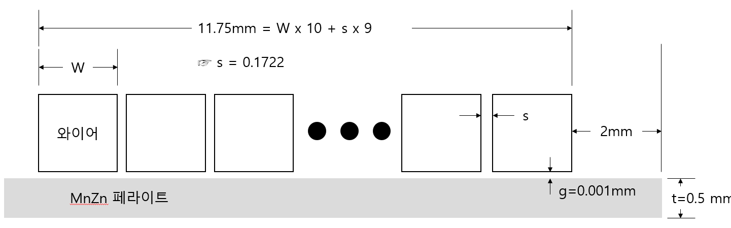
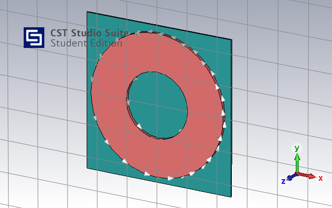
와이어는 통상 원형이나 해석을 간단하게 하기 위해서 정사각형 구조로 모델링한다. 이 경우 면적을 동일하게 하기 위해 폭을 계산한다. 요렇게 하는 것은 정확하지 않지만 모델링 쉽게 하고 해석시간을 단축시킬 수 있는 장점이 있다. 해석가능한 mesh수가 20,000개(테트라 메쉬)로 제한되어 있기 때문에 복잡한 구조는 해석이 안되니 참고 바란다.
Wires are usually circular, but for simplicity of interpretation, they are modeled as square structures. In this case, the width is calculated to equalize the area. This is inaccurate but has the advantage of making modeling easier and reducing analysis time. Please note that the number of meshes that can be analyzed is limited to 20,000 (tetra-mesh), so complex structures cannot be analyzed.

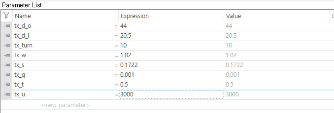
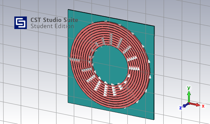
코일의 내경 20.5mm, 외경 44mm 구조를 감안하면 와이어간 간격을 대략 계산할 수 있다. 그리고 와이어와 페라이트간 절연이 필요하므로 물리적으로 0.001mm 거리를 둔다.
Given the coil's 20.5mm inside diameter and 44mm outside diameter construction, we can roughly calculate the spacing between the wires. And since we need insulation between the wires and the ferrite, we physically space them 0.001mm apart.
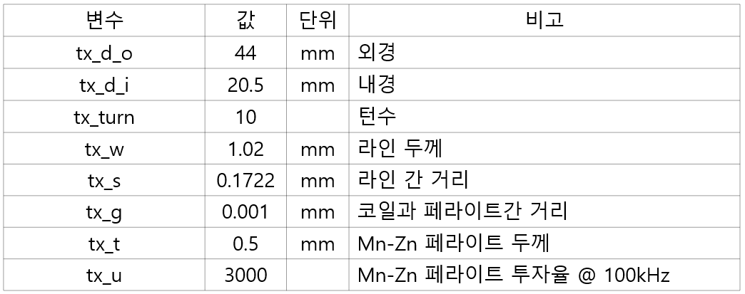
위에 설명된 것들을 정리하여 변수화 할 수 있도록 내용을 정리하면 아래와 같다.
To summarize the above so that we can make it variable, it looks like this.
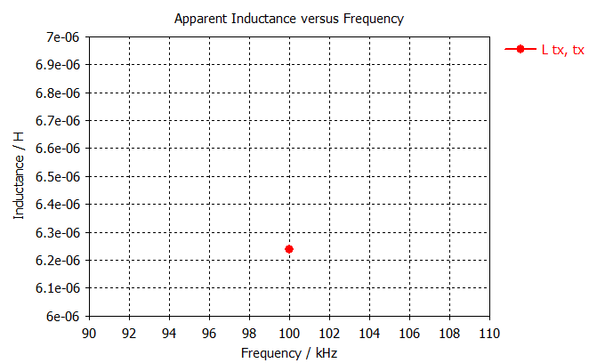
표준 문서를 보면 Ls (@100kHz)은 6.3uH 이다. 이를 기준으로 다양한 방식으로 해석 결과를 비교해 보자.
According to the standard document, Ls (@100kHz) is 6.3uH. Based on this, let's compare the results of various analyses.
1. Bulk Coil 형태로 해석하기(해석시간 짧음, 정확도 중)
1. Analyze as Bulk Coil (shortest analysis time, highest accuracy)
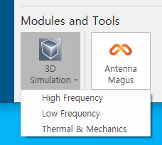
1-1 Low Frequency Solver로 새 프로젝트 시작, 파일 저장
1-1 Start a New Project with Low Frequency Solver, Save the File.
1-2. Unit 정의 : 길이 mm, 주파수 kHz, 온도 Celsius
1-2. Unit definitions: length mm, frequency kHz, temperature Celsius.

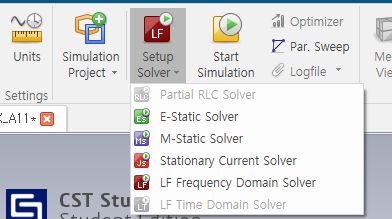
1-3. Solver 선택 : LF Frequency Domain Solver
1-3. Select Solver: LF Frequency Domain Solver
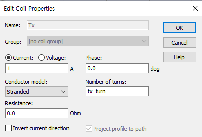
1-4. 변수 정의 및 값 입력
1-4. Define variables and enter values
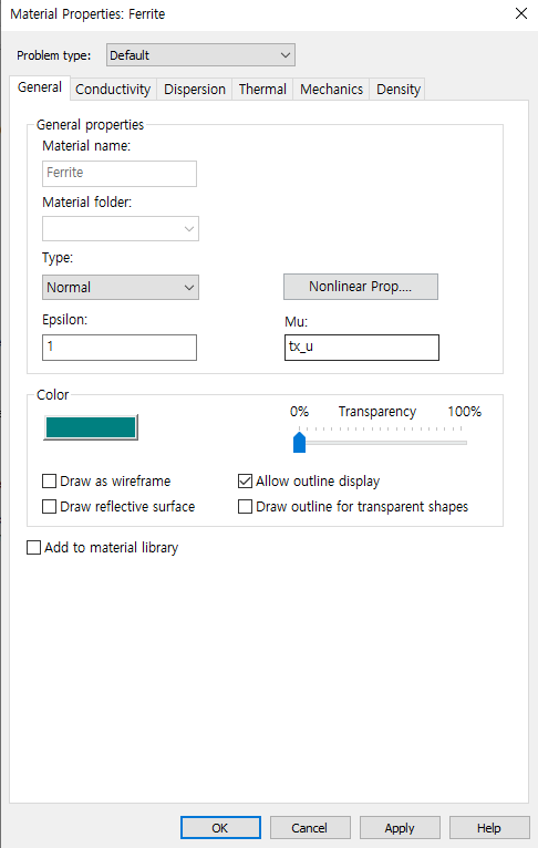
1-5. 페라이트 재질 지정하기
1-5. Specify the ferrite material
2. Bulk Coil 형태로 해석하기(해석시간 빠름, 인덕턴스 값 확인)
2. Analyze Bulk Coil shape (fast analysis time, check inductance value)

3. Ring Coil 형태로 해석하기(해석시간 보통, 정확도 중상)
3. Analyze as a ring coil (moderate analysis time, moderate accuracy)

4. Sprial Coil 형태로 해석하기(해석시간 긺, 정확도 상)
4. Analyze as a Sprial Coil (longer analysis time, higher accuracy)


5. 결론
5. conclusion
기본 3가지 방식으로 코일을 해석할 수 있다. A11의 사양은 L이 6.3uH이다. 위에서의 결과를 보면 경향성을 보고자 할 때는 모델링 쉽고 빠른 해석이 가능한 Bulk 모델(와이간 간격이 작을 때 추천)를 이용하면 좋고, 조금 더 정확히 볼 때는 Ring 모델로 단순화시키는 것이고, 정확하게 볼 때는 Spiral 모델로 보는 것이 좋은 것을 알 수 있다. 위의 결과는 Student Edition이기 때문에 Adaptive mesh를 적용하지 않고 기본 Mesh로만 해석하여 얻은 것이다.
There are three basic ways to interpret the coil. The A11 has a specification of L of 6.3uH. From the results above, we can see that if you want to see a trend, you can use the Bulk model (recommended when the wire spacing is small), which is easy to model and quick to analyze; if you want to be more precise, you can simplify to the Ring model; and if you want to be precise, you can use the Spiral model. The above results were obtained by solving with the default mesh without applying the Adaptive mesh because it is the Student Edition.
결합계수까지 구해 보려고 했으나 Mesh 수 제약으로 구할 수 없었다.
I also tried to get the coupling factor, but it was not possible due to the number of meshes.
결합계수 계산하기 위한 시뮬레이션
Simulation to Calculate Coupling Factors
CST STUDIO SUITE Learning Edition - Low Frequency Solver를 이용한 결합계수(Coupling Coefficient) 계산하기(Calculatio
기본적인 Coil의 인덕턴스(Self inductance)를 해석하는 것은 이전 글을 참조하기 바란다. https://mwave.tistory.com/312 CST STUDIO SUITE Learning Edition - Low Frequency Solver를 이용한 WPC Qi A11 Coil(Wireless Charging) 해석하
mwave.tistory.com
'과학기술 > Engineering Tools' 카테고리의 다른 글
| Ltspice를 이용한 Wireless Charging/Wireless Power Transfer 기본 회로 분석하기[2/3] - parameter sweep simulation (0) | 2022.12.23 |
|---|---|
| Ltspice를 이용한 Wireless Charging/Wireless Power Transfer 기본 회로 분석하기[1/3] - Basic simulation (0) | 2022.12.18 |
| Simulia Abaqus Learning Edition(학습용 버전) (0) | 2022.11.19 |
| Antenna Magus Learning Edition(학습용 버전) (0) | 2022.11.19 |
| Matlab을 대체하는 무료 프로그램 Octave, Scilab (0) | 2022.11.11 |


댓글