이번에는 Ltspice에서 Monte carlo simulation 하는 법을 소개한다.
This article will introduce how to do Monte carlo simulation in Ltspice.
방법은 아래 회로를 참고하여 보기 바란다. 함수 wc(값, 오차, 인덱스)와 함수 binary(실행, 인덱스) 정의한다.
Refer to the circuit below to see how. Define a function wc(value, error, index) and a function binary(execution, index).
즉 함수를 풀어보면 C2값은 2.2nF이고 1% 공차를 갖는 다면 wc(2.2nF, 0.022nF, index)가 될 것이다. 그리고 뒤에 인덱스는 변화를 가지고 적용해야 할 소자 수를 가리킨다. C2와 C3를 인덱스 2으로 놓아고 R3와 R4를 인덱스 1로 정의했는데 사실 제대로 하려면 소자별로 인덱스를 구분해야 한다. 그러면 총 인덱스는 4개가 되고 이에 대한 조합은 16개를 갖게 된다. 다만 여기서 해석을 줄이기 위해 동일한 소자가 적용된 것으로 가정하여 총 인덱스는 2개 이에 대한 조합은 4개로 정의한 것이다.
So if we solve the function and C2 is 2.2 nF and we have a 1% tolerance, we get wc(2.2 nF, 0.022 nF, index). The index after this is the number of elements to apply the change to. We put C2 and C3 as index 2 and defined R3 and R4 as index 1, but to do it right, we actually need to separate the indexes by element. This would give us a total of 4 indexes and 16 possible combinations. However, to simplify the interpretation, we assume that the same elements are applied, so we have defined a total index of 2 and 4 combinations.

상기 회로에서 Vds1 노드 즉 FET 스위치에 대한 전압이고 V(n002) 노드는 Coil과 공진 Cap. 사이의 전압을 보여준다.
In the above circuit, the Vds1 node is the voltage to the FET switch and the V(n002) node shows the voltage between the coil and the resonant Cap.

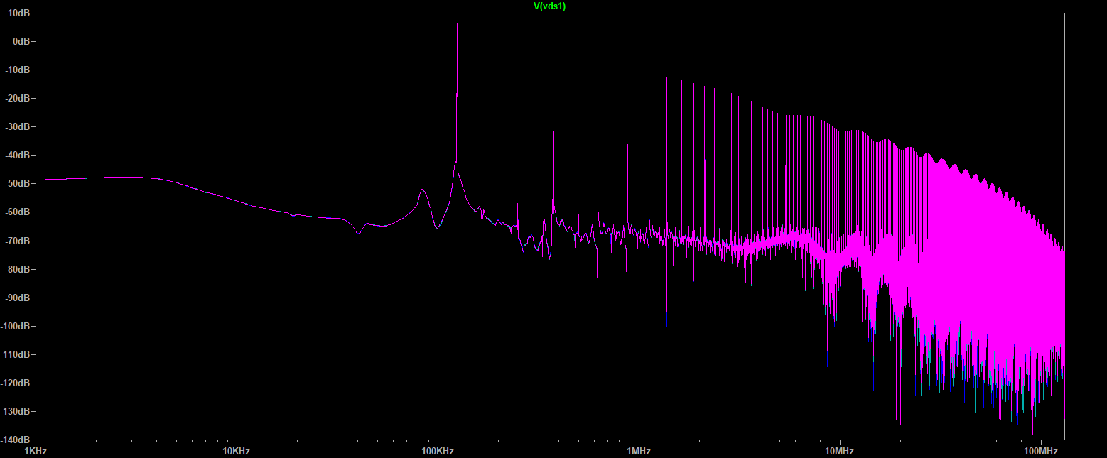
다음은 Vds1 노드의 전압을 가지고 FFT 처리한 결과를 본 것이다. 전압을 기준으로 FFT 처리를 하면 주파수 영역에서의 특성을 살펴볼 수 있다.
Here is the result of an FFT with the voltage of the Vds1 node. By FFTing the voltage, we can see the characteristics in the frequency domain.


댓글